How We Train Models at Clado
1) Context
Clado builds people search infrastructure, which involves indexing hundreds of millions of LinkedIn profiles and training models to first query and then filter through the rest to find the best matches for a natural language prompt. This is done with three models.
- Prompt -> Criteria (e.g., find me software engineers in sf -> is software engineer && is in sf)
- Criteria -> DSL (Elasticsearch Query)
- Our summer intern wrote a great blog on why the DSL step was necessary instead of just text2sql.
- Filtering. Given a profile, does it fulfill each criterion? Why or why not?
We trained custom models for each step, but I will ignore the first and third for the rest of this, since they were just simple fine-tuning on a GPT OpenSource model.
2) Constructing a Golden Dataset
We collect training data by mining real user prompts and turning them into trusted (prompt → DSL) pairs. A large “oracle” model (GPT-5) drafts the DSL, we run it against the database, and throw away anything that errors or returns obviously useless results. What’s left are labelled examples with the prompt, the accepted DSL, and a few basic stats (did it run, how many rows came back).
From there, we do a straightforward train-test split (70% for training, 30% held out to watch for overfitting), then fine-tune a GPT OSS 120B model with LoRA adapters. We rerun this workflow whenever the schema or user behavior changes, so the dataset stays fresh without manual labeling. The only metrics we track at this stage are simple: “does it run,” “is the result size reasonable,” and “did we include the obvious filters?” This gives us a labelled “golden dataset” to evaluate our search model against.
Side note: The better alternative to this synthetic approach is human labelled dataset, the risk of this approach is that we are blindly trusting the oracle model with a bit of scaffolding is the ground truth for this task. Unfortunately, we did not have the resources or time to generate a quality human label dataset.
3) Supervised Fine Tuning (Cold-Start)
Our RL loop is simple: for each prompt, we sample a few query → dsl pairs, run them, and rank the outputs. That costs real compute: every bad sample still hits the judge and often the database. If we start from an untrained model, most candidates don’t even run, so we burn cycles scoring garbage and get noisy learning signals.
Luckily, we can learn from Deepseeks' training runs for the R1; they found huge cost/compute savings by doing light supervised fine-tuning on a base model before starting RL.
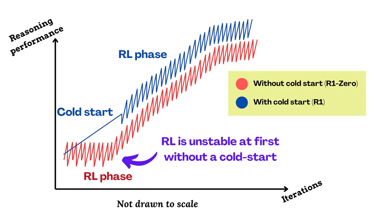
Diagram from this article explains this concept.
By first getting the model to produce mostly runnable, intent-matching DSL (via the golden set), RL spends its budget separating “good” from “better,” not “broken” from “barely usable.” That means fewer samples per prompt, fewer failed executions, more stable rewards, and faster convergence. Essentially, warming up the model so RL can focus on precision and coverage, not syntax.
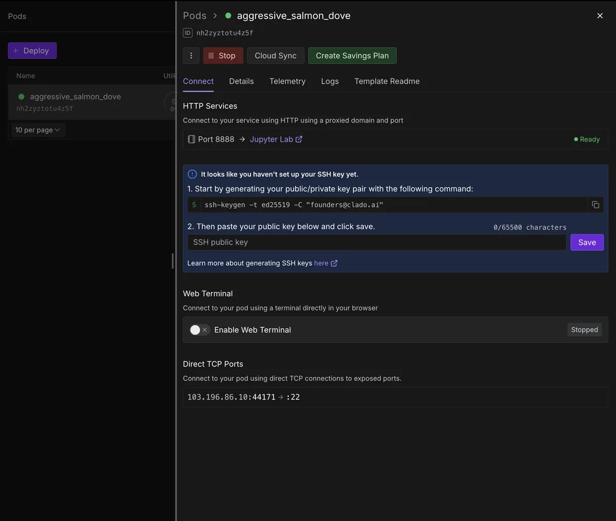 Rented 8xH100 on Runpod for all training
4) RL: Openpipe ART + RULER for rewards
In a nutshell: sample a few DSLs for a prompt, judge/rank them by how well they run and match intent, then nudge the model toward the better ones next time.
In practice (with OpenPipe ART), we train on small batches of real prompts (3 prompts/step). For each prompt, the model proposes 8 possible DSLs. Each DSL is executed; we also collect LLM-as-judge feedback. OpenPipe’s RULER combines these signals to rank candidates, and GRPO (group relative preference optimization) updates the model to prefer the higher-ranked ones.
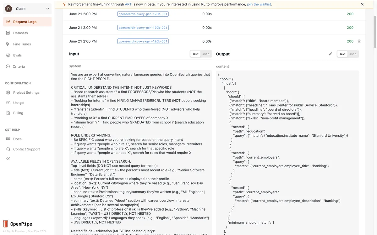 Sample Trajectory
The reward is practical: it would take into account whether the DSL executed (since we solved the cold start problem with SFT, this should mostly be in the clear), whether the results are relevant, and the quantity of results returned during the rollout. The following equation is a representation of the prompt that was put in RULER to calculate the quality of the DSL.
Why RULER:
RULER basically does the boring parts for you. It takes multiple signals (execution success, whether required filters were present, whether the query seems too broad, and an LLM-as-judge score) and combines them into a single ranking between “candidate A” and “candidate B.” That plugs directly into the policy optimization algorithm and in our case, GRPO.
You can skip RULER and just define a numeric reward yourself as a formula that mixes result count, coverage, penalties, etc. That gives you more direct control, and it’s nice because you can tune weights and see exactly why a query was rewarded. The downside is you end up rebuilding logic the judge is already doing (“is this actually relevant?”), and you still have to deal with edge cases like “query runs but is useless.”
In our case, most of the signal is already “prompt + LLM as a judge.” We’re not doing something like robotic control where the reward is purely numeric. So, letting RULER bundle those judge signals and rank candidates got us similar performance vs the hand-tuned formula.
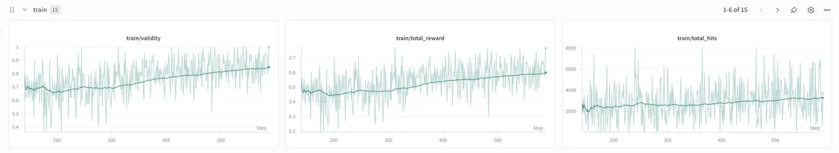 Loss over Training Steps
We keep the loop honest with lightweight observability in Weights & Biases: per-step win-rate vs. the baseline, execution success rate, histograms of result-set sizes (to catch over-broad queries), and simple regex/AST checks for missing WHEREs or bad joins.
5) Evals: Judgement Labs
We use an LLM as a judge to scale the non-deterministic part of evaluation (i.e., whether the final results match the user query) because labeled pairs are time-consuming to obtain. But every candidate also has to pass hard checks: the SQL must execute, obey the schema, and return a reasonable number of rows relative to the requested number.
Why this works: the premise of llm-as-judge seemed unintuitive to us at first, as we are essentially asking the same model to grade itself for completing the task. We assumed this would lead to heavy hallucination; however, this never occurred during training. Somehow, the models are better at grading problem sets than they are at solving them. The best explanation we have is that it is easier for a model to know if a Sudoku problem is solved, vs asking it to actually solve it (Credit to Alex Shan for this analogy).
Therefore, an eval is something we run that is powered by an LLM, along with quantitative equations that judge how good the results we returned are, combined with the number of results returned. For each model trained for a different purpose, a separate test is designed to provide a quantitative measure of how well the model performs. This algorithm/scorer can be used in production as well as with a testing set. At the end of every query, we would run a judge on the first five results and combine it with the total hits to understand how well we did for that specific query, then put it into buckets for further development and reference.
In addition, the scorer could also be used in conjunction with a testing set. To construct our evaluation testing set, we embedded all our customer queries, clustered them, and used the centroid of each cluster as our evaluation set to ensure the widest variety of results. This would help us decide whether to run RL on a newer model, since the scorer can also be applied to the base model to assess its performance. Furthermore, the eval can also help us determine whether the post-RL model actually performs better, since, due to inaccurate tuning, the resultant model can sometimes perform worse for reasons such as entropy collapse, KL collapse, or general reward hacking.
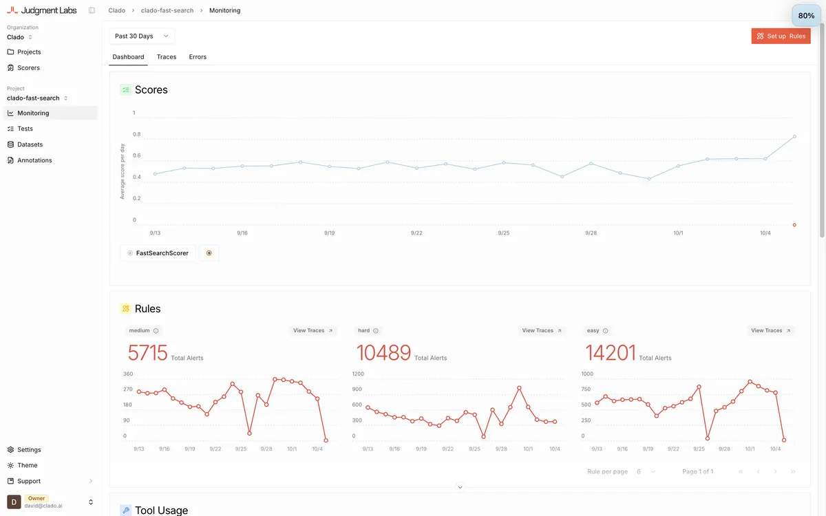 A snapshot of eval scores in Judgement Labs
We found that keeping a handful of “failed prompts” that once broke the system and plotting their pass rates across SFT → RL → APO was extremely helpful for catching drift.
6) Auto Prompt Optimization (DSPy)
After RL, we do a quick clean-up pass with DSPy to tune the system prompt for the Criteria→DSL model. We treat the prompt like parameters: compile new prompts, score them with the same signals we already trust (does the SQL execute, do we cover the required fields, what’s the RULER/judge score), and keep changes only if they help. We iterate until the gains plateau, with guardrails to prevent APO from drifting into behaviors RL has already fixed (e.g., re-introducing overly broad queries).
7) Results
GPT 120B Raw: 0.65, 639 tokens average, 10s average response time, $0.00016 average run cost
GPT 120B SFT + RL: 0.81, 448 tokens average, 7s average response time, $0.000112 average run cost
O3 raw: 0.72, 832 tokens average, 20.8s average response time, $0.006656 average run cost
For 300k runs O3 costs $1996.8, GPT 120B costs $33.6